By far, the greatest danger of Artificial Intelligence is that people conclude too early that they understand it.

Nowadays, creating a deep learning model is not a tough task anyone can get the boilerplate code and play around with it to create a model easily. But the main task lies in how to improve the model to be used in real use cases and can be put into production.

In this article, I will discuss some of the tips and tricks to be kept in mind while tweaking hyperparameters to make your model efficient and accurate.

Content

• Bias and Variance
• Stochastic vs Batch Learning
• Shuffling the Examples
• Normalizing the Inputs
• The Sigmoid
• Initializing the Weights
• Choosing Learning Rate

Before diving into the tricks directly Let's understand some basic terms beforehand.

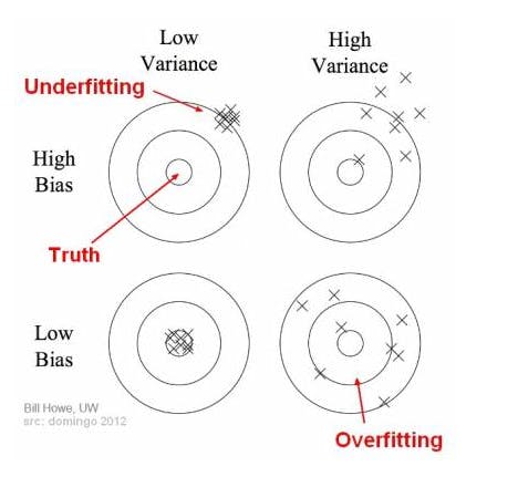
Bias and Variance

Bias is the measure of how much the network output averaged over all possible dataset differs from the desired output. In simple terms, we can define it as the difference between the average prediction of our model and the actual value which we are trying to predict. This is a measure to understand how well the model generalizes.

On the other hand, Variance is the variability of model prediction for a given data point. Variance can be determined by the spread of the prediction values for a model. If the prediction values are spread then we can say that the model has a high variation. Bias and Variance both contribute to the model accuracy.

In the initial phases of the training, bias is usually large as the model has just started to learn the parameters and thus can't generalize well during the initial phases of training. At the same time variance is very low as during the initial phases of training the data will have little influenced yet. Different phases of training will have varied Bias and Variance which can be understood by the figure below

1. Stochastic vs Batch Learning

Batch Learning requires a complete pass of the entire dataset in order to compute the gradient from which the weights are updated. On the other hand, In Stochastic Learning a single example is chosen randomly from the training set at each iteration. It means that the weight is updated after each iteration.

Why Stochastic Learning is Prefered over Batch Learning

• It is quite faster than batch learning.
• Stochastic Learning often leads to better solutions.
• Stochastic Learning can be used to track changes.

Some Advantages of Batch Learning

• The conditions of convergence(minimum) are well understood.
• Techniques such as conjugate gradient work only in batch learning.
• Weight Analysis, as well as convergence rates, are simple to determine. Solution:-

Stochastic Learning leads to a high change in the frequency of weight updation. Whereas It's impractical to perform batch learning. Another method to eliminate the drawbacks of both the method is Mini Batch learning. The concept of mini-batch is to start with small batch size and increase the size as the training proceeds.

2. Shuffling the Examples

A neural network learns the fastest from the examples i.e. unfamiliar to the system. Therefore, samples should be chosen in a way that the current batch should contain the examples that belong to different classes.

Another way is to first calculate the error between the predicted value and the ground truth value. The examples which give high error indicate that the corresponding input is not learned by the network. So, it makes sense to present the high error input frequently to the system so such patterns can also be learned well.

• Shuffle the training set so that the samples rarely belong to the same class.
• Present examples that produce large errors frequently compared to the ones with small errors.

3. Normalizing the Inputs

Convergence is usually faster in a neural network model if the average of training input is close to zero. So if our training data has all positive or all negative examples or both mixed then we can normalize it so that training will be faster.

• The average of each input variable over the training set should be close to zero.
• Scale input variables so that their covariance is almost the same.
• Input variable should not be co-related if possible.

4. The Sigmoid

In this section, every S-shaped graph represented by the activation function is said to be Sigmoid. We have basically two types of sigmoid:-

• Standard Logistic Function(also known as Sigmoid)
• Hyperbolic Tangent(also known as tanh)

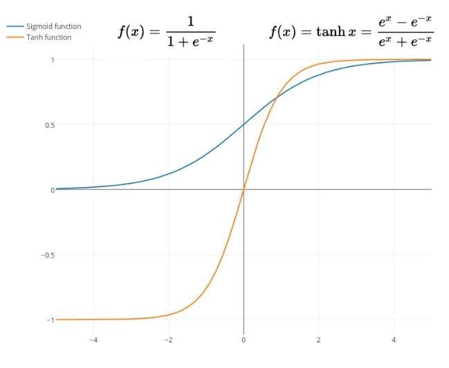
Key points:-

• tanh converge faster in comparison to sigmoids.
• A recommended tanh function is f(x) = 1.7159tanh(2/3x) as it is less expensive computationally.
• To avoid flat spots near to zero add small linear terms f(x)=tanh(x) + ax.

Note:- Nowadays RELU is preferred as a hidden layer in a neural network.

5. Initializing the Weights

The initial values of weight have a significant effect on the training process. Weights are chosen randomly but if the weight is chosen is too large it will lead to unstable learning. Too small weights also result in a slow training process, the network learns very slowly. Thus we should choose the appropriate weights to effectively train the neural network model. The performance can be measured if the chosen initial weights activate the linear part of the sigmoid.

• To achieve better results while training a model there should be coordination between the training set normalization, the choice of the sigmoid, and the initialization of the weights.

6. Choosing Learning Rate

Learning Rate is the parameter that decides the amount of the model weights to be updated during the training period. If the weight goes up and down frequently then the learning rate can be decreased whereas if the weights are quite stable then the learning rate can be increased. Mostly, the learning rates should be smaller for the initial layers of the network and greater for the latter layers of the network.

Equalizing the Learning Rates:-

• Give each weight its own learning rate.
• Learning Rate should be proportional to the square root of the number of inputs.
• Weights in later layers of the network should be larger than that of the initial layers.

Note:- Nowadays Adaptive Learning is used to update weight. In this method, the weights are updated according to the error calculated during each iteration. The speed of the learning rate is increased or decreased based on error.